Example notebook¶

This example will contain the following examples

Creating and saving a graph
Plotting the graph
Executing a node
Loading a graph from disk

Tip

Following this example requires familiarity with the core concepts of AutoDepGraph, we highly recommended to consult the (short) User guide before proceeding.

%matplotlib inline
import matplotlib.pyplot as plt
import networkx as nx
from importlib import reload
import os
import autodepgraph as adg
from autodepgraph import  AutoDepGraph_DAG

Creating a custom graph¶

A graph can be instantiated and nodes can be added to the graph as with any networkx graph object. It is important to specify a calibration_function.

cal_True_delayed =  'autodepgraph.node_functions.calibration_functions.test_calibration_True_delayed'
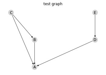
test_graph = AutoDepGraph_DAG('test graph')
for node in ['A', 'B', 'C', 'D', 'E']:
    test_graph.add_node(node,
                        calibrate_function=cal_True_delayed)

test_graph.add_node?

test_graph.add_edge('C', 'A')
test_graph.add_edge('C', 'B')
test_graph.add_edge('B', 'A')
test_graph.add_edge('D', 'A')
test_graph.add_edge('E', 'D')

Visualizing the graph¶

We support two ways of visualizing graphs: - matplotlib in the notebook - an svg in an html page that updates in real-time

Graphviz based SVG drawing of the graph¶

# The default plotting mode is SVG
test_graph.cfg_plot_mode = 'svg'
# Updates the monitor, in this case the svg/html page
test_graph.update_monitor()

# Updating the monitor overwrites an svg file whose location is determined by the attribute:
test_graph.cfg_svg_filename

'/home/docs/checkouts/readthedocs.org/user_builds/autodepgraph/envs/sphinx_doc/lib/python3.8/site-packages/autodepgraph/svg_viewer/adg_graph.svg'

from IPython.display import display, SVG
display(SVG(test_graph.cfg_svg_filename))

# The html page is located at the location specified by the url.
# The page generated based on a template when the open_html_viewer command is called.
# url = test_graph.open_html_viewer()
# print(url)

Matplotlib drawing of the graph¶

# Alternatively a render in matplotlib can be drawn
test_graph.draw_mpl()

Maintaining the graph¶

test_graph.set_all_node_states('needs calibration')

test_graph.maintain_B()

display(SVG(test_graph.cfg_svg_filename))

Maintaining node "B".
Maintaining node "A".
	Calibrating node A.

	Calibration of node A successful.
	Calibrating node B.

	Calibration of node B successful.

# Update the plotting monitor (default matplotlib) to show your graph
test_graph.update_monitor()

test_graph.set_all_node_states('needs calibration')

test_graph.maintain_node('E')

display(SVG(test_graph.cfg_svg_filename))

Maintaining node "E".
Maintaining node "D".
Maintaining node "A".
	Calibrating node A.

	Calibration of node A successful.
	Calibrating node D.

	Calibration of node D successful.
	Calibrating node E.

	Calibration of node E successful.

Three qubit example¶

This example shows a more realistic graph. The examples below show ways of exploring the graph

test_dir = os.path.join(adg.__path__[0], 'tests', 'test_data')
fn = os.path.join(test_dir, 'three_qubit_graph.yaml')
DAG = nx.readwrite.read_yaml(fn)

test_graph.cfg_plot_mode = 'svg'
DAG.update_monitor()
# This graph is so big, the html visualization is more suitable.
display(SVG(DAG.cfg_svg_filename))